Purpose
The main object of the chapter is to get acquainted with conceptual DB designing, justification of the relational data model choice, to provide brief information about the history of its creation, terminology and data structure, to present the description of relations on the stage of logic designing of relational database.
2.1. Conceptual DB designing
Actual DB designing (fig. 1.3) starts with conceptual modeling. This is general description that can be called DB scheme. The scheme is created by means of DBMS data definition language that was chosen for the project realization. It doesn’t give the possibility to present data in such way that created scheme can be understood by users of all categories
To resolve this problem data representation is realized by means of data model – integrated set of conceptions for its description, links between them and limitations [1, 2, 4, 6, 9…11]. It is necessary to guarantee that all participants of the project definitely understand rules of DB designing, types of available data processes, limitations that provides integration and guarantees correctness of data.
Conceptual DB designing is a choosing or creation of the technological process data representation model that doesn’t depend on any aspects of its physical location, organization and data processing [4].
Choosing or creation of data representation model is based on the analysis of requirements of the final system users. The model doesn’t depend on the type of DBMS that was chosen, set of application programs that were or will be created, programming language that is used, type of computer platform and etc. Data representation model that is a result of conceptual modeling is a source of information for logic DB designing stage. If each existing model (relational, network, hierarchical, object-oriented and etc.) is not good for use, in such case it is necessary to create own model of data presentation.
Hereinafter we’ll consider that according to the result of conceptional designing relational model was chosen because 80% of the up-to-date DBMS support just this model. And a lot of non-relational models are provided with user’s relational interface independently from basic data model that is used.
2.2. Relational model history
Relational model was first published by E.F. Codd in 1970 in the article “Relational data model for big shared data banks”. Publication of this article is considered to be a key point in the DB development history even though it is necessary to admit that another model based on multiplication was already proposed before (Childs, 1968) [1, 4, 6, 7, 9, 10, 12].
The reason of relational model creation includes 4 points [4]:
- To provide maximum possible level of data independence for application programs.
- To create firm basement for development of semantic issues and problems of consistency and data overflow.
- To expand data control language by including operations with ensembles.
The most significant researches of relational model’s capacity were carried out within the bounds of three projects.
First one was designed in the second half of 70s in the IBM corporation research laboratory, San Jose, California. The research was carried out by Astrahan. As the result installation “System R” was created. It was a prototype of true relational DBMS [12]. This project was designed to get practical proof of relational model’s usability. It became the most important source of information about such implementation problems as parallelism managing, requests optimization, transactions managing, providing data security and integrity, technology of renewing, considering human factor and designing of the user’s interface.
Implementation of the project created incentives for publication of many research scientific articles and creating many other prototypes of relational DBMS. This provided the possibility to [4]:
- firstly, create SQL data control language, sometimes spelled by means of mnemonic name “See-Quell”, that since has got status of formal ISO (International Organization for Standardization) standard and today is an actual branch standard of relational DBMS language;
- secondly, to create different commercial relational DBMS that first appeared on the market at the beginning of 80s, for example DB2 and SQL/DS, IBM corporation and ORACLE, ORACLE Corporation.
Another project that played a significant role in relational data model designing was INGRESS (Interactive Graphics Retrieval System) project. Work over this project was held in University of California, Berkeley nearly at the same time when System R project was in process. These researches caused creation of academic INGRESS version that made a significant contribution to the total recognition of relational data model. Latter INGRESS commercial products of Relational Technology Inc. (Ca-Open lngres, Computer Associates company nowadays) and Intelligent Database Machine, Britton Lee Inc. company branched off from this project.
The third project was Peterlee Relational Test Vehicle system of IBM research center, located in Peterly, Great Britain (Todd, 1976) [12]. This project was more theoretical than System R and INGRESS projects. Its results were extremely important especially for such branches as requests processing and optimization and functional development of the system [4].
Apart from this, later some extensions of relational data model were proposed. They were meant for complete and clear expression of data content (Codd, 1979), for the support of object-oriented conceptions (Stonebraker and Rowe, 1986), and also for support of deductive possibilities (Gardarin and Valduriez, 1989).
Thus, commercial systems on the base of relational data base began to appear at the end of 70s – beginning of 80s. For that period, several hundreds of different relational DBMS existed either for mainframes or for PC. However, most of them could not provide exact definition of relational data base. As an example of DBMS relational database for PC could be presented Oracle and MySQL (Oracle), Access, Foxpro, SQL-Server, Microsoft, InterBase (Embarcadero), Rbase (Microrim) DBMS and etc.
2.3. Data structure in relational model
2.3.1. Relations
Relational model is based on mathematical expression of relations [4, 6, 12, 13]. Let’s suppose, that we have two sets, D1 and D2, where D1={2,4} and D2={1,3,5}. Cartesian product of these two sets (denoted as D1 × D2) is a collection of all possible couples where the first element of set is D1, and second is an element of D2 set. The alternative method of this product calculation is search of all elements combinations, where the first element of set is D2, and second is an element of D1 set. As a result we get the following:
D1 × D2={(2, 1), (2, 3), (2, 5),(4, 1), (4,3), ( 4, 5)}.
Any subset of this Cartesian product is a relation. For example it is possible to single out R relations:
R = {(2, 1), (4, 1)}.
To find such possible couples that will be a part of relations, we can set any rules for sampling. For example, if to consider that relations R contain all possible couples that have second element equal to 1, the definition of relation R can be settled as following:
R = {(x, y),| x є D1, y є D2, y = 1}.
On the basis of the same sets we can form another relation – S, where the first element should always be twice bigger than a second one and the definition of relation S can be settled as following:
S = {(x, y),| x є D1, y є D2, x = 2 × y}.
In such case only one couple of the Cartesian product corresponds to this requirement:
S = {(2, 1)}.
Conception of relation can be easily expanded on three sets. Let’s suppose that we have three sets: – D1, D2 and D3. Cartesian product D1 × D2 × D3 of these three sets is a group that contains all possible groups of three elements, where first element of the set is D1, second one is an element of the set D2 and the thirds is an element of the set D3. Any subset of Cartesian product is relation. Let’s calculate Cartesian product of three sets D1={1,3}, D2={2,4} and D3={5,6}:
D1 × D2 × D3 = {(1, 2, 5), (1, 2, 6), (1, 4, 5), (1, 4, 6), (3, 2, 5), (3, 2, 6), (3, 4, 5), (3, 4, 6)}.
Any subset from given groups of three elements is a relation. Increasing the quantity of sets we can give a general definition of relation on n domains.
Let’s consider that we have n sets D1, D2, …, Dn. Cartesian product for these n sets can be defined as following:
D1 × D2 × … × Dn = {() | d<1 є D1, d<2 є D2, … d<n є Dn}.
Of course this expression is presented as:
Any set of n corteges of the Cartesian product is a relation between n sets. Pay attention that for the definition of these relations it is necessary to point out sets or domains that contain values for selection.
Physical representation of relations is a table.
Relations is a flat table that is composed from columns and rows.
Relations of the relational model is used to save the information about the subject (entity) that is presented in DB.
2.3.2. The description of relations structure
Attribute is a named column of relations.
Usually relation is a two-dimensional table, where rows correspond to separate records, and columns to attributes. Attributes can be put in any order – independently from their relocation relation will remain the same and thus will the same content. Each attribute of relational DB is determined in some document.
Domain is a set of probable values for one or several attributes.
Domains represent extremely powerful component of relational model. They can be different for each attribute, but two and more attributes can be determined on one domain. By means of domains user can reveal content and source of values that attributes get. As a result during the relational program running more information is available. It helps to avoid semantically illegal operations. For example it is useless to compare the author’s second name with the name of a book even if series of symbols are used as domains for both of these attributes. From the other side monthly rental for an object of property and quantity of months when it was hired, belong to different domains (the first attribute has monetary type, another one - integer-valued). However the multiplication of values from these domains is a possible operation. Relying on these two examples, it is not so easy to provide implementation of domain. That is why in many relational DBMS they get only partial support.
Tuples or rows of the table are the elements of relation. Corteges can be located in any order and relation will still be the same and thus have equal content.
Tuple is row of relation.
The description of relation structure together with domain specification and any other limitations of possible attributes values sometimes are called headline (or intension). Of course it is fixed as long as the content of relation is not changed by putting additional attributes. Tuples are called extension, state or body of relation that is changing continuously.
Relation rate is determined by quantity of contained attributes.
Relation with just one attribute has rate 1 and is called unary relation. Relations with two attributes are called binary, relations with three attributes are called ternary, and for relations with bigger quantity of attributes we use term n-ary. The definition of the relation rate is a part of a headline.
Cardinality is a quantity of tuples contained in relation.
This characteristic is changed with each addition or removal of tuples. Cardinality is a particularity of the relation’s body and is determined by current status of relation for arbitrary chosen moment.
2.3.3. Relational schema
Relational schema is a name of relation that reflects set of couples of attributes and domains.
For example, for attributes A1, A2, …, An with domains D1, D2, …, Dn the relational schema is a set {A1:D1, A2:D2, … An:Dn}. Relation R determined by relational schema S is a set that reflects attributes and correspondent domains names. Thus relation R is a multitude of such n-ary tuples {A1:d1, A2:d2, … An:dn}, where {d1:D1, d2:D2, … dn:Dn}.
Each element of n-tuple consists of attribute and its value. Usually for relation log presented as a table attribute names are listed in the headlines of columns. Tuples create rows of the format d1, d2, …, dn, where each value is taken from corresponding domain. Thus relations in relational model can be presented as random Cartesian product subset of domains’ attributes. Table – is just a physical reflection of such relation.
2.3.4. Characteristics of relations
- Relation has unique name in the DB.
- Each relation cell contains only indivisible values.
- Each attribute has unique name.
- Attribute’s value is taken from one domain.
- Order of domains can be random.
- Each relation tuple is unique.
- Theoretically the order of tuples location within relation is of no importance. (However in fact, this order can make a significant influence on data access efficiency.)
Most DB relations characteristics are based on mathematical relations.
- As relation is a set, the order of the elements is of no importance. Thus the tuples order in relation is insignificant.
- There are no iterative elements. So relation can not contain tuple-duplicates.
- To calculate of Cartesian product of sets with prime single-valued elements (for example integer-valued) each element in each tuple has single value. Similar to this each relation cell contains only one value. However, mathematical relation doesn’t need normalization. Codd proposed to prohibit the presence of iterative groups to simplify relational database model.
- The set of possible values for this position of relation is determined by set or domain. Relatively to DB all values in each attribute must come from domain that determined attribute.
However in mathematical relation the order of elements in tuple is of no importance. For example possible couple of values (1, 2) is rather different from possible couple of values (2, 1). This statement is not correct for relation model rate where it is specifically mentioned that the attributes order is insignificant. But if the structure of relation is already determined, the order of elements in tuples of its body should correspond to order of attributes’ names.
2.3.5. Relational keys
Relational keys are necessary for unique identification of each separate relations tuple according to its attributes’ value.
Super key is an attribute or a set of attributes that identifies in unique manner tuple of the relation.
As super key can contain additional attributes that are not necessary for unique identification of tuple, we will be interested in super keys that contain only those attributes that are really necessary for unique identification of tuples. So, super key can include several candidate keys.
Candidate key is a super key that doesn’t contain subsets and is a super key of the present relation. Relation can have several candidate keys.
If the key contains several attributes it is called compound key.
Candidate key for the present relation has two particularities.
Uniqueness. In each relation tuple the value of key identifies this tuple.
Minimal value. Each attribute can not be excluded from the key without breaking uniqueness.
Pay attention that any specific set of tuple relation can not be used to prove that some attribute or combination of attributes is a candidate key. The matter of fact that at some point there are no duplicate values doesn’t mean that there are no values at all. However, presence of duplicate values in some specific existing tuples set can be used to demonstrate that some combination of attributes can not be a candidate key. For the identification of candidate key it is necessary to know values of attributes that are used in “real world”. Only this point can ground the decision regarding the possibility of duplicate values existence. Considering only such kind of semantic information we can guarantee that some attributes combination is a relation candidate key.
Primary key is a candidate key that is chosen for unique identification of tuples within relation.
As relation doesn’t contain duplicate tuples, it is always possible to identify in unique way its each row. It means that relation always has primary key. In the worst case the whole set of attributes can be used as primary key, but of course to recognize tuples it is enough to use smaller set of attributes. Candidate keys that are not chosen to be primary key are called alternate keys.
Foreign key is an attribute or set of attributes within relation that corresponds to candidate key of some (or maybe the same) relation.
Relations that contain candidate key are called basic, target or parent relations. Relations with foreign key are called children relations.
2.3.6. Relational DB
Relational DB is a set of normalized relations.
Relational DB consists of relations. Structure of these relations is determined with special methods that are called normalization.
2.3.7. The description of relational data structure on different stages of designing
Model that presents data in terms of relational algebra that determines its structure, managing methods and providing data integrity is described on conceptual level. Any implementation of DBMS foresees that user interprets DB as a group of connected tables. Such perception has no attitude to the DB physical structure where the main point is an implementation on secondary media with indication of structure of saving and access methods that are used to organize efficient processing. On the stage of physical designing relations are called files, tuples are called records and attributes are called fields (fields) and etc. (see table. 2.1).
Table 2.1
Terms that describe relational model data structure | Conceptual design | Logical design | Physical design |
| Relation | Table | File |
| Tuple | Row | Log |
| Attribute | Column | Field |
| Relation rate | Number of columns | Number of fields |
| Cardinality | Number of rows | Number of logs |
| Key | Key | Index |
2.4. Logical DB designing
Logical DB designing is a process of DB scheme design (DB logic models) taking into consideration data presentation model that is independent of destination DBMS and other physical aspects of implementation [4, 6].
The objective of logical designing is creation of logic DB for the part of enterprise that is studied. Data presentation model that is determined on the stage of conceptual designing is a basis for logical data model that considers business processes of the company and their implementation in DBMS that was chosen. For example any particularities of physical organization of the data saving structure and index construction.
Logical model is a source of information for the stage of physical designing and it provides designer of physical DB the possibility to search for trade-offs that are necessary to reach the final object. It also plays an important role on the stage of operation and maintenance of the completed system. If the maintenance is organized duly, the actual logical database permits to present any modifications in the database obviously and clear. Also it gives the possibility to estimate its influence on application programs and usage of data that is present in the DB.
Logical model that represents particularities of enterprise work of many types of users at the same time is called global logical data model. There are two basic methods that permit to create global logical data model – centralized method and method of concept integration.
Centralized method lies in connection of requirements from separate users that are presented as different conceptions and thus make a united set of requirements received from all users that is used for global logical data model designing.
The particularity of such method is that lists of requirements are summarized till the creation of global logical data model. This method can be used only if DB is not too big or complicated.
Conception integration method lies in summarizing of separate local logical data models that represent conceptions of different groups of users in one global logical data model.
This method is more controllable as the whole work previously separated into smaller and easier for control parts. Of course difficulties arise if we try to unite local data models that were created by different designers that could use different terms for the same notions or quite the contrary – use one term for different conceptions.
DB logical designing is the most important stage that ensures the success of the whole system designing. If the designed project is not an exact representation of work methods and the enterprise structure, it will be very difficult or even impossible to determine all possible concepts (external schema) that are necessary for users or to organize the support of DB integrity. Also there can be some difficulties with physical implementation of DB or providing necessary efficiency of the system. At the same time the possibility of adaptation to the modifications is an attribute of well-designed DB. Thus it is worth spending some time and energy to create the best possible logical model.
2.5. Example of logical model
Let’s take a situation when you have got a task to create DB that permits to provide information about attending lessons. It is necessary to have the information about each student: how many hours of each subject were missed.
Let’s divide the information that is contained in DB into two groups: supplemental and on-line information. Then our registration DB will contain two lookup tables: “Students” and “Subjects”, and one table with supplemental information “Attendance” where we are going to list the information (fig.2.1.). It should be admitted that first of all it is necessary to set data in the tables with supplemental information, and after that to on-line information table.
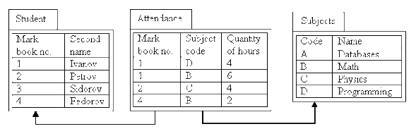
Fig.2.1. Attendance calculation database
Pay attention that in the column “Mark book no.” of the table “Attendance” only values from column “Mark book no.” of the table “Students” are mentioned. And in the column “Subject code” of the table “Attendance” only values from column “Code” of the table “Subjects” are mentioned. Thus it is possible to find the second name of a student according to the serial number of his mark book indicated in the table “Attendance”, and according to the code of a subject - to find out its name. From the other side it is possible to say how many students have never missed any lessons and what subject is attended by all students. Try to guess the name of a good student by yourself. Try to name the subject that is never missed.
While designing the DB always pay attention to the subject from both sides: from the position of designer and user. For designer it is important to input and receive the information from the DB easily and in digestible for user form. For user it is important to get the data in convenient form. It is not so easy to keep the balance of these interests. Especially, if the time of getting necessary information is limited.
The point of view of the DB designer is illustrated on the figure 2.1. Try to compose the table that illustrates how many lessons of each subject were missed by each student convenient to you by yourself. We will examine this task in the second half of our course when we study “Data representation”.
Such simplicity should not mislead you. Only the experience in DB designing will help you to create your own methods. In the proposed course conceptions and methods of DB designing are presented. It is useful to get acquainted with them.
- What is the objective of conceptual DB designing?
- What are the basic components of relational data structure?
- How Cartesian product and two-dimensional table are connected?
- What is included into the relation’s structure? What structure it has?
- What particularities of relations you know?
- Give the definition of relational keys that are familiar to you.
- What particularities of candidate key you can name?
- What is the main purpose of DB logical designing?
- Compare methods of logical DB model.
Conclusion
Conception of relational data organization proved its vitality in practice, as it occupied about 80% of the world’s DBMS market. Flexible methods of relational database logical modeling provides demonstrable implementation easy and extremely complicated business processes for a large circle of users that have different skills.