Purpose
The purpose of the chapter is to present basic information about relational algebra as a theoretical language of operations.
Relational algebra is a theoretical language of operations the permits to create on the basis of one or two relations another relation without changing output data [1, 4, 6, 7, 9, 10, 12].
Both operands and product are relations, and thus outcomes of one operation can become output data for another operation. This gives the possibility to create nested expressions of relational algebra the same way as arithmetic expressions are built. This is called a property closure. That means that relations are covered by relational algebra the same as numbers by arithmetic operations [4].
Relational algebra is a language of sequential relations usage where all corteges, even taken from different relations, are processed by one command without loop organization. For commands of relational algebra there are several syntax options. Below we will apply generally used character expressions of these commands and present them in an informal form. More detailed information on this question an interested reader can find in the papers of Ullman, 1988.
There are several options of operations selection that are included into relational algebra. First Codd proposed to eight operators, but later were added some more. Five basic operations of relational algebra (fig.5.1.) are: selection, projection, cartesian product, union and set difference. They use most operations of data access that can be interesting for us. On the vase of five principal operations it is possible to deduce additional operations (fig. 5.1): join, intersection and division.
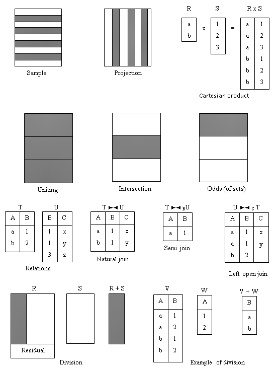
Fig. 5.1. Scheme of relational algebra operators functions representation
Access and projection operations are unary as they work with one relation. Other operations work with couples of relations and that is why they are called binary operations. In the given below definitions R and S – these are two relations that are determined on the attributes A = (a1, a2, …, an) and B = (b1, b2, …, bn) correspondingly. To illustrate the results of the operations execution we will use «LIBRARY» DB relations (appendix B).
5.2. Sample (or limitation)
| σпредикат(R) | Sample operation works with only one relation R and determines final relation that contains only corteges (row) of relation R that meet given task (predicate). |
EXAMPLE 5.1
Compose a list of librarians who have clock number that exceeds 80.
σClockNumber > 80 (Librarians)
Outcome relation is the relation Librarians, and predicate is an expression ClockNumber>80. Sample operation determines new relation that contains only those corteges of relation Librarians,, where ClockNumber attribute value exceeds 80 (table 5.1). More complicated predicates can be created by means of logic operators AND, OR or NOT.
Table 5.1
The result of sample operation implementation for Librarians relation | Code | ClockNumber | FamilyName | Name | Patronymic | PasportCode | Post | HomePhone | Note |
| 3 | 187 | Inozemtseva | Ivanna | Modestovna | 9 | Senior Librarian | 775-XX-00 | null |
| 4 | 83 | Malzeva | Diana | Petrovna | 12 | Librarian | 29-XX-15 | null |
| 6 | 100 | Stavka | Lidia | Ivanovna | 7 | Librarian | 22-XX-01 | null |
| Патр 1, …, атр n (R) | Operation of projection works with only one relation R and determines new relation that includes vertical subset of R relation that is created by sample of indicated attributes values and deletion of row-duplicates products. |
EXAMPLE 5.2
Compose a list of librarians that contains clock number value (ClockNumber), familyname (FamilyNamе), name (Name), patronymic (Patronymic) and home telephone (HomePhone).
ПClockNumber, FamilyName, Name, Patronymic, HomePhone (R)
In this example, application operations of projection determines new relation that will contain only attributes ClockNumber, FamilyNamе, Name, Patronymic and HomePhone of relation Librarians, put in indicated order (table 5.2).
Table 5.2
The projection of Librarians relation | ClockNumber | FamilyName | Name | Patronymic | HomePhone |
| 28 | Ivanova | Alena | Vladimirovna | 52-XX-75 |
| 12 | Nikolaenko | Lubov | Nikolaevna | 46-XX-19 |
| 187 | Inozemtseva | Ivanna | Modestovna | 775-XX-00 |
| 83 | Malzeva | Diana | Petrovna | 29-XX-15 |
| 10 | Sizranzeva | Tatyana | Igorevna | 370-XX-22 |
| 100 | Stavka | Lilia | Ivanovna | 22-XX-01 |
| 50 | Leshenko | Alla | Fedorovna | 722-XX-36 |
| 36 | Sira | Lidia | Ivanovna | 254-XX-02 |
| 45 | Prokhina | Tamara | Lvovna | 63-XX-01 |
| 78 | Samilenko | Viktoria | Igorevna | 125-XX-80 |
| 69 | Stepanova | Aleksandra | Nikolaevna | 445-XX-65 |
| 17 | Petrova | Alina | Sergeevna | 999-XX-05 |
| R × S | Operation of Cartesian product determines new relation that is an outcome of concatenation (that is chaining) of each cortege of relation R with each cortege of relation S. |
Sample and projection operators carry out data mining from one relation only. Can arise the situation when some combination of data from several relations is necessary. Operator of Cartesian product multiplies two relations. As a result we get new relation that contains all possible cortege couples from both relations. Thus if one relation has I corteges and N attributes and another one J corteges and M attributes, the relation with its Cartesian product will contain (I × J) corteges and (N + M) attributes. Outcome relations can have attributes with the same names. In such case attributes names will contain names of relations as prefixes. This guarantees uniqueness of attribute names in the result relation.
EXAMPLE 5.3
Compose a list of all readers who have ever taken books in the library using the following attributes of relation Readers: Code, FamilyName, Name and relation BookGiveOutRecord: Code, ReaderCode, InventoryCode.
(ПCode, FamilyName, Name (Readers)) × (ПCode, ReaderCode, InventoryCode(BookGiveOutRecord))
The product of carrying out such operation is a relation that contain 120 corteges and 6 attributes. There is no sense to illustrate its complete version. Look at first 12 corteges (table 5.3.). First 10 represent all possible combinations of the first cortege of relation Readers with ten corteges of relation BookGiveOutRecord. Two last positions are presented to compare their values with first two rows. These are two first possible combinations of the second cortege of relation Readers with first two corteges of relation BookGiveOutRecord. Next one will be third possible combination of the second cortege Readers with third cortege of relation BookGiveOutRecord. And then up till n-th cortege.
Table 5.3
Cartesian relation of Reader and BookGiveOutRecord relations | Readers.Code | FamilyName | Name | BookGiveOutRecord.Code | ReaderCode | InventoryCode |
| 1 | Ivanov | Petr | 1 | 2 | 6 |
| 1 | Ivanov | Petr | 2 | 3 | 4 |
| 1 | Ivanov | Petr | 3 | 6 | 3 |
| 1 | Ivanov | Petr | 4 | 4 | 6 |
| 1 | Ivanov | Petr | 5 | 7 | 7 |
| 1 | Ivanov | Petr | 6 | 9 | 12 |
| 1 | Ivanov | Petr | 7 | 11 | 10 |
| 1 | Ivanov | Petr | 8 | 7 | 8 |
| 1 | Ivanov | Petr | 9 | 9 | 12 |
| 1 | Ivanov | Petr | 10 | 12 | 15 |
| 2 | Fedorez | Irina | 1 | 2 | 6 |
| 2 | Fedorez | Irina | 2 | 3 | 4 |
In such form (120 corteges) this relation contains more information than necessary. For example first cortege of this relation contains different values of attributesReaders.Code and ReaderCode. To get necessary list (table 5.4) we should make a sample of corteges that meet equality Readers.Code = ReaderCode. Completely this operation looks asfollowing:
σReaders.Code = ReaderCode (ПCode, FamilyName, Name(Readers)) × (ПCode, ReaderCode, InventoryCode(BookGiveOutRecord))
Table 5.4
Bounded Cartesian product of relations Reader і BookGiveOutRecord | Readers.Code | FamilyName | Name | BookGiveOutRecord.Code | ReaderCode | InventoryCode |
| 2 | Fedorez | Irina | 1 | 2 | 6 |
| 3 | Ilin | Ivan | 2 | 3 | 4 |
| 6 | Nosenko | Oleg | 3 | 6 | 3 |
| 4 | Surenko | Dmitry | 4 | 4 | 6 |
| 7 | Brusov | Vladimir | 5 | 7 | 7 |
| 9 | Levchenko | Julia | 6 | 9 | 12 |
| 11 | Sheglov | Petr | 7 | 11 | 10 |
| 7 | Brusov | Vladimir | 8 | 7 | 8 |
| 9 | Levchenko | Julia | 9 | 9 | 12 |
| 12 | Kirilenko | Viktor | 10 | 12 | 15 |
As we are going to see later, combination of Cartesian product and sample can be reduced to one operation - uniting.
| R ∪ S | Uniting of relations R and S with corteges I and J correspondingly we cam get after their concatenation with creation of one relation with maximal quantity of corteges (I + J) if corteges-duplicates are deleted. In such case relations R and S must be compatible to unite. |
Uniting of relations is possible only in case if their schemes concur, that is if they have equal quantity of attributes with domains (types of data) that concur. Such relations are compatible to unite. We should mention that in some cases to get two compatible relations the projection operation can be used.
EXAMPLE 5.4
Compose the list of familynames of all people that are mentioned in the DB.
ПFamilyName(Readers) U ПFamilyName(Librarians)
To create compatible relations first of all it is necessary to apply projection operation so that it is possible to delete from relations Readers and Librarians columns with attributes FamilyName, including duplicates if necessary. After that to combine received intermediate relations operation of uniting should be used (Table 5.5).
Table 5.5
The result of uniting relations Readers and Librarians according to attribute FamilyName | FamilyName |
| Brusov |
| Ilin |
| Inozemtseva |
| Ivanov |
| Ivanova |
| Fedorez |
| Kirilenko |
| Korshunova |
| Kozirev |
| Leshenko |
| Levchenko |
| Malzeva |
| Nikolaenko |
| Nosenko |
| Petrova |
| Prokhina |
| Samojlenko |
| Sheglov |
| Sira |
| Sizranzeva |
| Stavka |
| Stepanova |
| Surenko |
| Svetlaya |
| R - S | Difference between relations R and S is composed of corteges that are present in relation R, but are absent in relation S. At the same time relations R and S must be compatible for uniting. |
EXAMPLE 5.5
Determine individual codes of readers who have never taken books it the library.
ПCode(Readers) – ПReaderCode(BookGiveOutRecord)
In this case, the same as for previous one, it is necessary to create integrated relation Readers and BookGiveOutRecord. Their projection must be executed according to the attributes Code and ReaderCode. Then we have to apply the operation of difference (Table 5.6).
Table 5.6
Difference between relations Readers and BookGiveOutRecord | Code |
| 1 |
| 5 |
| 8 |
| 10 |
Usually users are interested only in some part of all combinations of Cartesian product corteges that meets determined requirements. That is why instead of Cartesian product only one of the most important operations of relational algebra is applied – operation of integration. The result of its running on the base of two initial relations new relation is created. Operation of integration is derivative from Cartesian product operation. It is equal to Cartesian product sample operation of two relations with corteges that meet requirement determined in the predicate of integration. Predicate of integration is an equivalent. From position of effective implementation in relational DBMS this operation is one of the most complicated and is usually the main reason that causes efficiency problems that are typical for all relational systems.
Let’s study the following kinds of join:
- Θ-join.
- equi-join (separate kind of theta join).
- Natural join.
- Outer join.
- Semi-join.
5.7.1. Θ-join
| R►◄FS | Operation of Θ-join determines relation that contains corteges of Cartesian product of relations R and S, that meet predicate F. Predicate F is presented as R.aiΘS.bi, where instead of Θ can be used one of comparison operators (<, <=,>, >=, =, ≈). |
Symbol of theta join can be represented on the platform of basic operations of sample and Cartesian product:
The same as for cartesian product, the degree of theta join is defined as sum of operand-relations R and S degrees. If predicate F is contained only in operators of equality (=), then this is an equi-join.
EXAMPLE 5.6
Compose the list of all readers that have ever taken books in the library (table 5.4).
In example that illustrates Cartesian product to receive this list Cartesian product and sample operations were applied. However the same result can be achieved by means of equi-join operation.
(ПCode, FamilyName, Name(Readers))►◄Readers.Code = ReaderCode(ПCode, ReaderCode, InventoryCode(BookGiveOutRecord))
5.7.2. Natural joint
| R►◄S | Natural joint is a joint implemented according to equivalence of two relations R and S, carried out according to all general attributes x. One sample of each shared attribute is excluded from the result of natural joint. |
The degree of natural joint is a sum of R and S operands-relations degrees minus quantity of x attributes. In the example of theta join equi-join was used to compose this list. There were present two attributes, Readers.Code and ReaderCode, that contain codes of library readers. If they would have the same name, for example ReaderCode, it might be possible to apply natural join operation to delete one of them.
EXAMPLE 5.7
Compose the list of all readers that have even taken books in the library (table 5.7).
(ПReaderCode, FamilyName, Name(Readers))►◄(ПCode, ReaderCode, InventoryCode(BookGiveOutRecord))
Table 5.7
Natural join of relations Readers and BookGiveOutRecord | ReaderCode | FamilyName | Name | BookGiveOutRecord.Code | InventoryCode |
| 2 | Fedorez | Irina | 1 | 6 |
| 3 | Ilin | Ivan | 2 | 4 |
| 6 | Nosenko | Oleg | 3 | 3 |
| 4 | Surenko | Dmitry | 4 | 6 |
| 7 | Brusov | Vladimir | 5 | 7 |
| 9 | Levchenko | Julia | 6 | 12 |
| 11 | Sheglov | Petr | 7 | 10 |
| 7 | Brusov | Vladimir | 8 | 8 |
| 9 | Levchenko | Julia | 9 | 12 |
| 12 | Kirilenko | Victor | 10 | 15 |
5.7.3. Outer join
Usually, when two relations are joined, the cortege of one relation can not find corresponding cortege in another relation. In other words, distinct values can be found in the columns of join. It can be necessary that the row of one relation is represented in the join result even if there is no concurrent value. This can be achieved by outer join.
To indicate absent values in the result join NULL determinant is applied. The advantage of outer join is saving of output information: corteges that are lost when other types of join are implemented.
| R⊃◄S | Left outer join is a join where corteges of relation R that has no concurrent values in the columns shared with relation S are also included to result relation. |
EXAMPLE 5.8
To indicate code, family name, name, patronymic for all readers and information from BookGiveOutRecord for those who took books in the library (table 5.8).
(ПCode, FamilyName, Name, Patronymic(Readers))⊃◄(ПOutLibrarianCode, InventoryCode, IssueDate, ReturnDate, FactReturnDate, InLibrarianCode(BookGiveOutRecord))
Strictly speaking, in the example left (natural) outer join is illustrated, as all corteges of left relation are contained in the result relation. Also there is a right outer join that received its name because all corteges of right join are contained in the result relation. Apart from it there is a complete outer join, where the result join contains all corteges from both relations and NULL determinant is used to indicate distinct values of corteges.
Table 5.8
Left outer join of relations Readers and BookGiveOutRecord projection | ReaderCode | FamilyName | Name | Patronymic | OutLibrarianCode | InventoryCode | IssueDate | ReturnDate | FactReturnDate | InLibrarianCode |
| 1 | Ivanov | Petr | Ivanovich | NULL | NULL | NULL | NULL | NULL | NULL |
| 2 | Fedorez | Irina | Olegovna | 4 | 6 | 11.09.2004 | 25.09.2004 | 24.09.2004 | 3 |
| 3 | Ilin | Ivan | Petrovich | 4 | 4 | 02.09.2004 | 16.09.2004 | 11.12.2004 | 3 |
| 4 | Surenko | Dmitry | Pavlovich | 3 | 6 | 30.10.2004 | 13.11.2004 | 10.01.2005 | 6 |
| 5 | Korshunova | Natalia | Yurievna | NULL | NULL | NULL | NULL | NULL | NULL |
| 6 | Nosenko | Oleg | Vladimirovitch | 4 | 3 | 02.09.2004 | 16.09.2004 | 16.09.2004 | 1 |
| 7 | Brusov | Vladimir | Mikhajlovitch | 9 | 8 | 07.03.2009 | 21.03.2009 | 10.04.2009 | 10 |
| 7 | Brusov | Vladimir | Mikhajlovitch | 10 | 7 | 10.11.2009 | 24.11.2009 | 24.11.2009 | 12 |
| 8 | Kozirev | Alexey | Sergeevich | NULL | NULL | NULL | NULL | NULL | NULL |
| 9 | Levchenko | Julia | Pavlovna | 7 | 12 | 15.12.2009 | 29.12.2009 | NULL | 9 |
| 9 | Levchenko | Julia | Pavlovna | 8 | 12 | 05.02.2010 | 29.02.2010 | NULL | 11 |
| 10 | Svetlaya | Tatyana | Ivanovna | NULL | NULL | NULL | NULL | NULL | NULL |
| 11 | Sheglov | Petr | Yevgenievich | 8 | 10 | 06.02.2009 | 20.02.2009 | 19.02.2009 | 7 |
| 12 | Kirilenko | Victor | Alexandrovich | 10 | 15 | 21.09.2010 | 05.10.2010 | 03.10.2010 | 9 |
5.7.4. Semi-join
| R►FS | Semi-join operation determines relation that contains those corteges of relation R that are included in R and S relations join. |
The advantage of semi-join is that it permits to reduce the quantity of corteges that must be processed for join. It is particularly useful for joins computing in the distributed systems. Semi-join operation can be defined by means of projection and join operators:
Where A is a set of all attributes of relation R. In fact this is a half-theta-join and it is necessary to admit that there are semi-joins of equivalence and half-natural join.
EXAMPLE 5.9
Compose a report that includes complete information about all readers with name «Dmitry» who have ever taken books in the library (table 5.9).
Readers►Readers.Code = BookGiveOutRecord.ReaderCode AND Reader.Name = ‘Dmitry’BookGiveOutRecord
Table 5.9
Readers and BookGiveOutRecord relations semi-join result | Code | FamilyName | Name | Patronymic | ReaderCardNumber | PasportCode | Job | Post | Note |
| 4 | Surenko | Dmitry | Pavlovich | 543 | 6 | NMU, geophysicst dep. | Senior professor | NULL |
| R ∩ S | Operation of intersection determines relation that contains corteges that are present in relation R the same as in relation S. Relations R and S must be compatible for join. |
Intersection can be noted down using operator of deference of sets: R ∩ S= R – (R – S).
EXAMPLE 5.10
Compose the list of librarians who are readers at the same time. Indicate their passport code, family name, name and patronymic.
(ПPasportCode, FamilyName, Name, Patronymic(Readers)) ∩ (ПPasportCode, FamilyName, Name, Patronymic(Librarians))
To use the terms of compatibility for join of relations that intersect the corresponding operations of projection were implemented.
Data that are set into relations «READERS» and «LIBRARIANS» (appendix B) prove that the result of their join is a null set that means that non of librarians is a reader.
Operator of division can be useful in case of special queries that can be carried pout rather often. Let’s consider that relation R is determined on the set of attributes A, and relation S – on the set of attributes B. At the same time B ⊆ A (that means that B is a subset of A). Let C =A - B, that means that C is a set of R relation attributes that is not attributes of relation S. Then definition of division operator can be presented as following:
| R ÷ S | The result of division operator is a set of R relation corteges defined according to the set of C attributes that meet the combination of all relation S corteges. |
This operator can be noted down using other basic operators:
T1 = ПC(R)
T2 = ПC((S × T1) – R)
T = T1 – T2
EXAMPLE 5.11
Create a list of names, surnames, patronymic names and passport codes of readers born after December 1, 1960.
R = ПCode, PassportCode, FamilyName, Name, Patronymic(Readers) (табл. 5.10);
S = ПCode(σBirthday > 31.12.1960(PasportData)) (table 5.11);
R ÷ S = (ПCode, PassportCode(Readers)) ÷ (ПCode(σBirthday > 31.12.1960(PasportData))) (table 5.12).
For the solution of the task, it is first necessary to obtain the relation R. To do this, a projection of the relation Readers is performed (table 5.10). Then we have to determine the relation S. For this, the projection of the relation PasportData is defined. In it, using the sampling operator, all passport codes with a date of birth after December 31, 1960 (table 5.11) were found. Now we can to obtain the result of dividing the relation R by the relation S (table 5.12).
Table 5.10
Relation R | Code | PasportCode | FamilyName | Name | Patronymic |
| 1 | 4 | Ivanov | Petr | Ivanovich |
| 2 | 1 | Fedorez | Irina | Olegovna |
| 3 | 11 | Ilin | Ivan | Petrovich |
| 4 | 6 | Surenko | Dmitry | Pavlovich |
| 5 | 8 | Korshunova | Natalia | Yurievna |
| 6 | 5 | Nosenko | Oleg | Vladimirovitch |
| 7 | 24 | Brusov | Vladimir | Mikhajlovitch |
| 8 | 15 | Kozirev | Alexey | Sergeevich |
| 9 | 18 | Levchenko | Julia | Pavlovna |
| 10 | 22 | Svetlaya | Tatyana | Ivanovna |
| 11 | 14 | Sheglov | Petr | Yevgenievich |
| 12 | 17 | Kirilenko | Victor | Alexandrovich |
Table 5.11
Relation S | Code |
| 3 |
| 5 |
| 7 |
| 8 |
| 12 |
| 14 |
| 15 |
| 16 |
| 18 |
| 19 |
| 20 |
| 21 |
| 22 |
| 23 |
| 24 |
Table 5.12
Product R ÷ S | PasportCode | FamilyName | Name | Patronymic |
| 8 | Korshunova | Natalia | Yurievna |
| 5 | Nosenko | Oleg | Vladimirovitch |
| 24 | Brusov | Vladimir | Mikhajlovitch |
| 15 | Kozirev | Alexey | Sergeevich |
| 18 | Levchenko | Julia | Pavlovna |
| 22 | Svetlaya | Tatyana | Ivanovna |
| 14 | Sheglov | Petr | Yevgenievich |
- What particularities of relational algebra you know?
- What operations of relational algebra you know?
- What is the difference between sample and projection operations?
- Which one of two relations will contain more attributes and corteges, if the first one is a Cartesian product of relations R, of I corteges and N attributes, and S, with J corteges and M attributes, and the second relation is a join of the same relations?
- Give the definition of the operations of relational algebra that need compatible for join output relations?
- What operations of relational algebra derivative from Cartesian product you know?
- Which comparison operator converts Θ-join into natural join?
- What is the difference between outer and inner joins?
- How is generated relation that is a product of familiar to you out join type work?
Conclusion
Syntax of SQL-operators, that are applied for data processing in relational DBMS of different designers, can differ, but operations of relational algebra is a mathematical basement that units them. In case of necessity this fact can be useful to convert DB of relational DBMS that is applied for resolving current tasks of organization into the format of another designer.